8.1 graph 
This module implements two-dimensional linear and logarithmic graphs,
including automatic scale and tick selection (with the ability to
override manually). A graph is a guide (that can be drawn with
the draw command, with an optional legend) constructed with one of
the following routines:
guide graph(picture pic=currentpicture, real f(real), real a, real b,
            int n=ngraph, real T(real)=identity,
            interpolate join=operator --);
guide[] graph(picture pic=currentpicture, real f(real), real a, real b,
             int n=ngraph, real T(real)=identity, bool3 cond(real),
             interpolate join=operator --);
return a graph using the scaling information for picturepic(see automatic scaling) of the functionfon the interval [T(a),T(b)], sampling atnpoints evenly spaced in [a,b], optionally restricted by the bool3 functioncondon [a,b]. Ifcondis:true, the point is added to the existing guide;default, the point is added to a new guide;false, the point is omitted and a new guide is begun.
The points are connected using the interpolation specified by
join:-
operator --(linear interpolation; the abbreviationStraightis also accepted); -
operator ..(piecewise Bezier cubic spline interpolation; the abbreviationSplineis also accepted); -
linear(linear interpolation), Hermite(standard cubic spline interpolation using boundary conditionnotaknot,natural,periodic,clamped(real slopea, real slopeb)), ormonotonic. The abbreviationHermiteis equivalent toHermite(notaknot)for nonperiodic data andHermite(periodic)for periodic data).
guide graph(picture pic=currentpicture, real x(real), real y(real),
            real a, real b, int n=ngraph, real T(real)=identity,
            interpolate join=operator --);
guide[] graph(picture pic=currentpicture, real x(real), real y(real),
              real a, real b, int n=ngraph, real T(real)=identity,
              bool3 cond(real), interpolate join=operator --);
returns a graph using the scaling information for picturepicof the parametrized function (x(t),y(t)) for t in the interval [T(a),T(b)], sampling atnpoints evenly spaced in [a,b], optionally restricted by the bool3 functioncondon [a,b], using the given interpolation type.guide graph(picture pic=currentpicture, pair z(real), real a, real b, int n=ngraph, real T(real)=identity, interpolate join=operator --); guide[] graph(picture pic=currentpicture, pair z(real), real a, real b, int n=ngraph, real T(real)=identity, bool3 cond(real), interpolate join=operator --);returns a graph using the scaling information for picturepicof the parametrized functionz(t) for t in the interval [T(a),T(b)], sampling atnpoints evenly spaced in [a,b], optionally restricted by the bool3 functioncondon [a,b], using the given interpolation type.guide graph(picture pic=currentpicture, pair[] z, interpolate join=operator --); guide[] graph(picture pic=currentpicture, pair[] z, bool3[] cond, interpolate join=operator --);returns a graph using the scaling information for picturepicof the elements of the arrayz, optionally restricted to those indices for which the elements of the boolean arraycondaretrue, using the given interpolation type.guide graph(picture pic=currentpicture, real[] x, real[] y, interpolate join=operator --); guide[] graph(picture pic=currentpicture, real[] x, real[] y, bool3[] cond, interpolate join=operator --);returns a graph using the scaling information for picturepicof the elements of the arrays (x,y), optionally restricted to those indices for which the elements of the boolean arraycondaretrue, using the given interpolation type.-
guide polargraph(picture pic=currentpicture, real f(real), real a,
                 real b, int n=ngraph, interpolate join=operator --);
returns a polar-coordinate graph using the scaling information for picturepicof the functionfon the interval [a,b], sampling atnevenly spaced points, with the given interpolation type. guide polargraph(picture pic=currentpicture, real[] r, real[] theta, interpolate join=operator--);returns a polar-coordinate graph using the scaling information for picturepicof the elements of the arrays (r,theta), using the given interpolation type.
An axis can be drawn on a picture with one of the following commands:
void xaxis(picture pic=currentpicture, Label L="", axis axis=YZero,
           real xmin=-infinity, real xmax=infinity, pen p=currentpen,
           ticks ticks=NoTicks, arrowbar arrow=None, bool above=false);
Draw an x axis on picturepicfrom x=xminto x=xmaxusing penp, optionally labelling it with LabelL. The relative label location along the axis (a real number from [0,1]) defaults to 1 (see Label), so that the label is drawn at the end of the axis. An infinite value ofxminorxmaxspecifies that the corresponding axis limit will be automatically determined from the picture limits. The optionalarrowargument takes the same values as in thedrawcommand (see arrows). The axis is drawn before any existing objects inpicunlessabove=true. The axis placement is determined by one of the followingaxistypes:YZero(bool extend=true)¶Request an x axis at y=0 (or y=1 on a logarithmic axis) extending to the full dimensions of the picture, unless
extend=false.YEquals(real Y, bool extend=true)¶Request an x axis at y=
Yextending to the full dimensions of the picture, unlessextend=false.Bottom(bool extend=false)¶Request a bottom axis.
Top(bool extend=false)¶Request a top axis.
BottomTop(bool extend=false)¶Request a bottom and top axis.
Custom axis types can be created by following the examples in the module
graph.asy. One can easily override the default values for the standard axis types:import graph; YZero=new axis(bool extend=true) { return new void(picture pic, axisT axis) { real y=pic.scale.x.scale.logarithmic ? 1 : 0; axis.value=I*pic.scale.y.T(y); axis.position=1; axis.side=right; axis.align=2.5E; axis.value2=Infinity; axis.extend=extend; }; }; YZero=YZero();The default tick option is
NoTicks. The optionsLeftTicks,RightTicks, orTickscan be used to draw ticks on the left, right, or both sides of the path, relative to the direction in which the path is drawn. These tick routines accept a number of optional arguments:ticks LeftTicks(Label format="", ticklabel ticklabel=null, bool beginlabel=true, bool endlabel=true, int N=0, int n=0, real Step=0, real step=0, bool begin=true, bool end=true, tickmodifier modify=None, real Size=0, real size=0, bool extend=false, pen pTick=nullpen, pen ptick=nullpen);If any of these parameters are omitted, reasonable defaults will be chosen:
-
Label format¶ override the default tick label format (
defaultformat, initially "$%.4g$"), rotation, pen, and alignment (for example,LeftSide,Center, orRightSide) relative to the axis. To enable LaTeX math mode fonts, the format string should begin and end with$see format. If the format string istrailingzero, trailing zeros will be added to the tick labels; if the format string is"%", the tick label will be suppressed;ticklabelis a function
string(real x)returning the label (by default, format(format.s,x)) for each major tick valuex;bool beginlabelinclude the first label;
bool endlabelinclude the last label;
int Nwhen automatic scaling is enabled (the default; see automatic scaling), divide a linear axis evenly into this many intervals, separated by major ticks; for a logarithmic axis, this is the number of decades between labelled ticks;
int ndivide each interval into this many subintervals, separated by minor ticks;
real Stepthe tick value spacing between major ticks (if
N=0);real stepthe tick value spacing between minor ticks (if
n=0);bool begininclude the first major tick;
bool endinclude the last major tick;
tickmodifier modify;an optional function that takes and returns a
tickvaluestructure having real[] membersmajorandminorconsisting of the tick values (to allow modification of the automatically generated tick values);real Sizethe size of the major ticks (in
PostScriptcoordinates);real sizethe size of the minor ticks (in
PostScriptcoordinates);bool extend;extend the ticks between two axes (useful for drawing a grid on the graph);
pen pTickan optional pen used to draw the major ticks;
pen ptickan optional pen used to draw the minor ticks.
For convenience, the predefined tickmodifiers
OmitTick(...real[] x),OmitTickInterval(real a, real b), andOmitTickIntervals(real[] a, real[] b)can be used to remove specific auto-generated ticks and their labels. TheOmitFormat(string s=defaultformat, ... real[] x)ticklabel can be used to remove specific tick labels but not the corresponding ticks. The tickmodifierNoZerois an abbreviation forOmitTick(0)and the ticklabelNoZeroFormatis an abbreviation forOmitFormat(0).It is also possible to specify custom tick locations with
LeftTicks,RightTicks, andTicksby passing explicit real arraysTicksand (optionally)tickscontaining the locations of the major and minor ticks, respectively:ticks LeftTicks(Label format="", ticklabel ticklabel=null, bool beginlabel=true, bool endlabel=true, real[] Ticks, real[] ticks=new real[], real Size=0, real size=0, bool extend=false, pen pTick=nullpen, pen ptick=nullpen)void yaxis(picture pic=currentpicture, Label L="", axis axis=XZero, real ymin=-infinity, real ymax=infinity, pen p=currentpen, ticks ticks=NoTicks, arrowbar arrow=None, bool above=false, bool autorotate=true);Draw a y axis on picturepicfrom y=yminto y=ymaxusing penp, optionally labelling it with a LabelLthat is autorotated unlessautorotate=false. The relative location of the label (a real number from [0,1]) defaults to 1 (see Label). An infinite value ofyminorymaxspecifies that the corresponding axis limit will be automatically determined from the picture limits. The optionalarrowargument takes the same values as in thedrawcommand (see arrows). The axis is drawn before any existing objects inpicunlessabove=true. The tick type is specified byticksand the axis placement is determined by one of the followingaxistypes:XZero(bool extend=true)¶Request a y axis at x=0 (or x=1 on a logarithmic axis) extending to the full dimensions of the picture, unless
extend=false.XEquals(real X, bool extend=true)¶Request a y axis at x=
Xextending to the full dimensions of the picture, unlessextend=false.Left(bool extend=false)¶Request a left axis.
Right(bool extend=false)¶Request a right axis.
LeftRight(bool extend=false)¶Request a left and right axis.
-
For convenience, the functions
void xequals(picture pic=currentpicture, Label L="", real x,
             bool extend=false, real ymin=-infinity, real ymax=infinity,
             pen p=currentpen, ticks ticks=NoTicks, bool above=true,
             arrowbar arrow=None);
and
void yequals(picture pic=currentpicture, Label L="", real y,
             bool extend=false, real xmin=-infinity, real xmax=infinity,
             pen p=currentpen, ticks ticks=NoTicks, bool above=true,
             arrowbar arrow=None);
can be respectively used to call
yaxisandxaxiswith the appropriate axis typesXEquals(x,extend)andYEquals(y,extend). This is the recommended way of drawing vertical or horizontal lines and axes at arbitrary locations. void axes(picture pic=currentpicture, Label xlabel="", Label ylabel="", bool extend=true, pair min=(-infinity,-infinity), pair max=(infinity,infinity), pen p=currentpen, arrowbar arrow=None, bool above=false);This convenience routine draws both x and y axes on picturepicfrommintomax, with optional labelsxlabelandylabeland any arrows specified byarrow. The axes are drawn on top of existing objects inpiconly ifabove=true.void axis(picture pic=currentpicture, Label L="", path g, pen p=currentpen, ticks ticks, ticklocate locate, arrowbar arrow=None, int[] divisor=new int[], bool above=false, bool opposite=false);This routine can be used to draw on picturepica general axis based on an arbitrary pathg, using penp. One can optionally label the axis with LabelLand add an arrowarrow. The tick type is given byticks. The optional integer arraydivisorspecifies what tick divisors to try in the attempt to produce uncrowded tick labels. Atruevalue for the flagoppositeidentifies an unlabelled secondary axis (typically drawn opposite a primary axis). The axis is drawn before any existing objects inpicunlessabove=true. The tick locatorticklocateis constructed by the routineticklocate ticklocate(real a, real b, autoscaleT S=defaultS, real tickmin=-infinity, real tickmax=infinity, real time(real)=null, pair dir(real)=zero);where
aandbspecify the respective tick values atpoint(g,0)andpoint(g,length(g)),Sspecifies the autoscaling transformation, the functionreal time(real v)returns the time corresponding to the valuev, andpair dir(real t)returns the absolute tick direction as a function oft(zero means draw the tick perpendicular to the axis).- These routines are useful for manually putting ticks and labels on axes
(if the variable
Labelis given as theLabelargument, theformatargument will be used to format a string based on the tick location):void xtick(picture pic=currentpicture, Label L="", explicit pair z, pair dir=N, string format="", real size=Ticksize, pen p=currentpen); void xtick(picture pic=currentpicture, Label L="", real x, pair dir=N, string format="", real size=Ticksize, pen p=currentpen); void ytick(picture pic=currentpicture, Label L="", explicit pair z, pair dir=E, string format="", real size=Ticksize, pen p=currentpen); void ytick(picture pic=currentpicture, Label L="", real y, pair dir=E, string format="", real size=Ticksize, pen p=currentpen); void tick(picture pic=currentpicture, pair z, pair dir, real size=Ticksize, pen p=currentpen); void labelx(picture pic=currentpicture, Label L="", explicit pair z, align align=S, string format="", pen p=currentpen); void labelx(picture pic=currentpicture, Label L="", real x, align align=S, string format="", pen p=currentpen); void labelx(picture pic=currentpicture, Label L, string format="", explicit pen p=currentpen); void labely(picture pic=currentpicture, Label L="", explicit pair z, align align=W, string format="", pen p=currentpen); void labely(picture pic=currentpicture, Label L="", real y, align align=W, string format="", pen p=currentpen); void labely(picture pic=currentpicture, Label L, string format="", explicit pen p=currentpen);
Here are some simple examples of two-dimensional graphs:
-
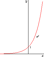
This example draws a textbook-style graph of
y= exp(x), with the y axis starting at y=0:
import graph;
size(150,0);

real f(real x) {return exp(x);}
pair F(real x) {return (x,f(x));}

draw(graph(f,-4,2,operator ..),red);

xaxis("$x$");
yaxis("$y$",0);

labely(1,E);
label("$e^x$",F(1),SE);
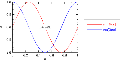
- The next example draws a scientific-style graph with a legend.
The position of the legend can be adjusted either explicitly or by using the
graphical user interface (see Graphical User Interface). If an
UnFill(real xmargin=0, real ymargin=xmargin)orFill(pen)option is specified toadd, the legend will obscure any underlying objects. Here we illustrate how to clip the portion of the picture covered by a label:import graph; size(400,200,IgnoreAspect); real Sin(real t) {return sin(2pi*t);} real Cos(real t) {return cos(2pi*t);} draw(graph(Sin,0,1),red,"$\sin(2\pi x)$"); draw(graph(Cos,0,1),blue,"$\cos(2\pi x)$"); xaxis("$x$",BottomTop,LeftTicks); yaxis("$y$",LeftRight,RightTicks(trailingzero)); label("LABEL",point(0),UnFill(1mm)); add(legend(),point(E),20E,UnFill);
To specify a fixed size for the graph proper, use
attach:import graph; size(250,200,IgnoreAspect); real Sin(real t) {return sin(2pi*t);} real Cos(real t) {return cos(2pi*t);} draw(graph(Sin,0,1),red,"$\sin(2\pi x)$"); draw(graph(Cos,0,1),blue,"$\cos(2\pi x)$"); xaxis("$x$",BottomTop,LeftTicks); yaxis("$y$",LeftRight,RightTicks(trailingzero)); label("LABEL",point(0),UnFill(1mm)); attach(legend(),truepoint(E),20E,UnFill);A legend can have multiple entries per line:
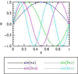
import graph;
size(8cm,6cm,IgnoreAspect);

typedef real realfcn(real);
realfcn F(real p) {
  return new real(real x) {return sin(p*x);};
}

for(int i=1; i < 5; ++i)
  draw(graph(F(i*pi),0,1),Pen(i),
       "$\sin("+(i == 1 ? "" : (string) i)+"\pi x)$");
xaxis("$x$",BottomTop,LeftTicks);
yaxis("$y$",LeftRight,RightTicks(trailingzero));

attach(legend(2),(point(S).x,truepoint(S).y),10S,UnFill);
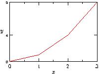
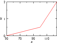
- This example draws a graph of one array versus another (both of
the same size) using custom tick locations and a smaller font size for
the tick labels on the y axis.
import graph;

size(200,150,IgnoreAspect);

real[] x={0,1,2,3};
real[] y=x^2;

draw(graph(x,y),red);

xaxis("$x$",BottomTop,LeftTicks);
yaxis("$y$",LeftRight,
      RightTicks(Label(fontsize(8pt)),new real[]{0,4,9}));
- This example shows how to graph columns of data read from a file.
import graph;

size(200,150,IgnoreAspect);

file in=input("filegraph.dat").line();
real[][] a=in;
a=transpose(a);

real[] x=a[0];
real[] y=a[1];

draw(graph(x,y),red);

xaxis("$x$",BottomTop,LeftTicks);
yaxis("$y$",LeftRight,RightTicks);
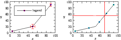
- The next example draws two graphs of an array of coordinate pairs,
using frame alignment and data markers. In the left-hand graph, the
markers, constructed with
marker marker(path g, markroutine markroutine=marknodes,
              pen p=currentpen, filltype filltype=NoFill,
              bool above=true);
using the path
unitcircle(see filltype), are drawn below each node. Any frame can be converted to a marker, usingmarker marker(frame f, markroutine markroutine=marknodes, bool above=true);In the right-hand graph, the unit n-sided regular polygon
polygon(int n)and the unit n-point cyclic crosscross(int n, bool round=true, real r=0)(whereris an optional “inner” radius) are used to build a custom marker frame. Heremarkuniform(bool centered=false, int n, bool rotated=false)adds this frame atnuniformly spaced points along the arclength of the path, optionally rotated by the angle of the local tangent to the path (if centered is true, the frames will be centered withinnevenly spaced arclength intervals). Alternatively, one can use markroutinemarknodesto request that the marks be placed at each Bezier node of the path, or markroutinemarkuniform(pair z(real t), real a, real b, int n)to place marks at pointsz(t)for n evenly spaced values oftin[a,b].These markers are predefined:
marker[] Mark={
  marker(scale(circlescale)*unitcircle),
  marker(polygon(3)),marker(polygon(4)),
  marker(polygon(5)),marker(invert*polygon(3)),
  marker(cross(4)),marker(cross(6)),marker(diamond),marker(plus);
};

marker[] MarkFill={
  marker(scale(circlescale)*unitcircle,Fill),marker(polygon(3),Fill),
  marker(polygon(4),Fill),marker(polygon(5),Fill),
  marker(invert*polygon(3),Fill),marker(diamond,Fill)
};
The example also illustrates the
errorbarroutines:void errorbars(picture pic=currentpicture, pair[] z, pair[] dp, pair[] dm={}, bool[] cond={}, pen p=currentpen, real size=0); void errorbars(picture pic=currentpicture, real[] x, real[] y, real[] dpx, real[] dpy, real[] dmx={}, real[] dmy={}, bool[] cond={}, pen p=currentpen, real size=0);Here, the positive and negative extents of the error are given by the absolute values of the elements of the pair array
dpand the optional pair arraydm. Ifdmis not specified, the positive and negative extents of the error are assumed to be equal.import graph; picture pic; real xsize=200, ysize=140; size(pic,xsize,ysize,IgnoreAspect); pair[] f={(5,5),(50,20),(90,90)}; pair[] df={(0,0),(5,7),(0,5)}; errorbars(pic,f,df,red); draw(pic,graph(pic,f),"legend", marker(scale(0.8mm)*unitcircle,red,FillDraw(blue),above=false)); scale(pic,true); xaxis(pic,"$x$",BottomTop,LeftTicks); yaxis(pic,"$y$",LeftRight,RightTicks); add(pic,legend(pic),point(pic,NW),20SE,UnFill); picture pic2; size(pic2,xsize,ysize,IgnoreAspect); frame mark; filldraw(mark,scale(0.8mm)*polygon(6),green,green); draw(mark,scale(0.8mm)*cross(6),blue); draw(pic2,graph(pic2,f),marker(mark,markuniform(5))); scale(pic2,true); xaxis(pic2,"$x$",BottomTop,LeftTicks); yaxis(pic2,"$y$",LeftRight,RightTicks); yequals(pic2,55.0,red+Dotted); xequals(pic2,70.0,red+Dotted); // Fit pic to W of origin: add(pic.fit(),(0,0),W); // Fit pic2 to E of (5mm,0): add(pic2.fit(),(5mm,0),E);
-
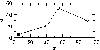
A custom mark routine can be also be specified:
import graph;

size(200,100,IgnoreAspect);

markroutine marks() {
  return new void(picture pic=currentpicture, frame f, path g) {
    path p=scale(1mm)*unitcircle;
    for(int i=0; i <= length(g); ++i) {
      pair z=point(g,i);
      frame f;
      if(i % 4 == 0) {
        fill(f,p);
        add(pic,f,z);
      } else {
        if(z.y > 50) {
          pic.add(new void(frame F, transform t) {
              path q=shift(t*z)*p;
              unfill(F,q);
              draw(F,q);
            });
        } else {
          draw(f,p);
          add(pic,f,z);
        }
      }
    }
  };
}

pair[] f={(5,5),(40,20),(55,51),(90,30)};

draw(graph(f),marker(marks()));

scale(true);

xaxis("$x$",BottomTop,LeftTicks);
yaxis("$y$",LeftRight,RightTicks);
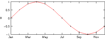
- This example shows how to label an axis with arbitrary strings.
import graph;

size(400,150,IgnoreAspect);

real[] x=sequence(12);
real[] y=sin(2pi*x/12);

scale(false);

string[] month={"Jan","Feb","Mar","Apr","May","Jun",
                "Jul","Aug","Sep","Oct","Nov","Dec"};

draw(graph(x,y),red,MarkFill[0]);

xaxis(BottomTop,LeftTicks(new string(real x) {
      return month[round(x % 12)];}));
yaxis("$y$",LeftRight,RightTicks(4));
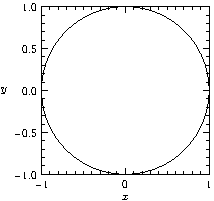
- The next example draws a graph of a parametrized curve.
The calls to
xlimits(picture pic=currentpicture, real min=-infinity,
        real max=infinity, bool crop=NoCrop);
and the analogous function
ylimitscan be uncommented to set the respective axes limits for picturepicto the specifiedminandmaxvalues. Alternatively, the functionvoid limits(picture pic=currentpicture, pair min, pair max, bool crop=NoCrop);
can be used to limit the axes to the box having opposite vertices at the given pairs). Existing objects in picture
picwill be cropped to lie within the given limits ifcrop=Crop. The functioncrop(picture pic)can be used to crop a graph to the current graph limits.import graph; size(0,200); real x(real t) {return cos(2pi*t);} real y(real t) {return sin(2pi*t);} draw(graph(x,y,0,1)); //limits((0,-1),(1,0),Crop); xaxis("$x$",BottomTop,LeftTicks); yaxis("$y$",LeftRight,RightTicks(trailingzero));
The function
guide graphwithderiv(pair f(real), pair fprime(real), real a, real b,
                     int n=ngraph#10);
can be used to construct the graph of the parametric function
fon[a,b]with the control points of thenBezier segments determined by the specified derivativefprime:unitsize(2cm); import graph; pair F(real t) { return (1.3*t,-4.5*t^2+3.0*t+1.0); } pair Fprime(real t) { return (1.3,-9.0*t+3.0); } path g=graphwithderiv(F,Fprime,0,0.9,4); dot(g,red); draw(g,arrow=Arrow(TeXHead));

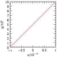
The next example illustrates how one can extract a common axis scaling factor.
import graph;

axiscoverage=0.9;
size(200,IgnoreAspect);

real[] x={-1e-11,1e-11};
real[] y={0,1e6};

real xscale=round(log10(max(x)));
real yscale=round(log10(max(y)))-1;

draw(graph(x*10^(-xscale),y*10^(-yscale)),red);

xaxis("$x/10^{"+(string) xscale+"}$",BottomTop,LeftTicks);
yaxis("$y/10^{"+(string) yscale+"}$",LeftRight,RightTicks(trailingzero));
Axis scaling can be requested and/or automatic selection of the axis limits can be inhibited with one of these
scaleroutines:void scale(picture pic=currentpicture, scaleT x, scaleT y); void scale(picture pic=currentpicture, bool xautoscale=true, bool yautoscale=xautoscale, bool zautoscale=yautoscale);This sets the scalings for picture
pic. Thegraphroutines accept an optionalpictureargument for determining the appropriate scalings to use; if none is given, it uses those set forcurrentpicture.Two frequently used scaling routines
LinearandLogare predefined ingraph.All picture coordinates (including those in paths and those given to the
labelandlimitsfunctions) are always treated as linear (post-scaled) coordinates. Usepair Scale(picture pic=currentpicture, pair z);
to convert a graph coordinate into a scaled picture coordinate.
The x and y components can be individually scaled using the analogous routines
real ScaleX(picture pic=currentpicture, real x);
real ScaleY(picture pic=currentpicture, real y);
The predefined scaling routines can be given two optional boolean arguments:
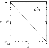
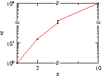
automin=falseandautomax=automin. These default tofalsebut can be respectively set totrueto enable automatic selection of "nice" axis minimum and maximum values. TheLinearscaling can also take as optional final arguments a multiplicative scaling factor and intercept (for a depth axis,Linear(-1)requests axis reversal).For example, to draw a log/log graph of a function, use
scale(Log,Log):import graph; size(200,200,IgnoreAspect); real f(real t) {return 1/t;} scale(Log,Log); draw(graph(f,0.1,10)); //limits((1,0.1),(10,0.5),Crop); dot(Label("(3,5)",align=S),Scale((3,5))); xaxis("$x$",BottomTop,LeftTicks); yaxis("$y$",LeftRight,RightTicks);
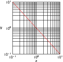
By extending the ticks, one can easily produce a logarithmic grid:
import graph;
size(200,200,IgnoreAspect);

real f(real t) {return 1/t;}

scale(Log,Log);
draw(graph(f,0.1,10),red);
pen thin=linewidth(0.5*linewidth());
xaxis("$x$",BottomTop,LeftTicks(begin=false,end=false,extend=true,
                                ptick=thin));
yaxis("$y$",LeftRight,RightTicks(begin=false,end=false,extend=true,
                                 ptick=thin));
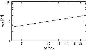
One can also specify custom tick locations and formats for logarithmic axes:
import graph;

size(300,175,IgnoreAspect);
scale(Log,Log);
draw(graph(identity,5,20));
xlimits(5,20);
ylimits(1,100);
xaxis("$M/M_\odot$",BottomTop,LeftTicks(DefaultFormat,
                                        new real[] {6,10,12,14,16,18}));
yaxis("$\nu_{\rm upp}$ [Hz]",LeftRight,RightTicks(DefaultFormat));
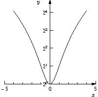
It is easy to draw logarithmic graphs with respect to other bases:
import graph;
size(200,IgnoreAspect);

// Base-2 logarithmic scale on y-axis:

real log2(real x) {static real log2=log(2); return log(x)/log2;}
real pow2(real x) {return 2^x;}

scaleT yscale=scaleT(log2,pow2,logarithmic=true);
scale(Linear,yscale);

real f(real x) {return 1+x^2;}

draw(graph(f,-4,4));

yaxis("$y$",ymin=1,ymax=f(5),RightTicks(Label(Fill(white))),EndArrow);
xaxis("$x$",xmin=-5,xmax=5,LeftTicks,EndArrow);
Here is an example of "broken" linear x and logarithmic y axes that omit the segments [3,8] and [100,1000], respectively. In the case of a logarithmic axis, the break endpoints are automatically rounded to the nearest integral power of the base.
import graph;

size(200,150,IgnoreAspect);

// Break the x axis at 3; restart at 8:
real a=3, b=8;

// Break the y axis at 100; restart at 1000:
real c=100, d=1000;

scale(Broken(a,b),BrokenLog(c,d));

real[] x={1,2,4,6,10};
real[] y=x^4;

draw(graph(x,y),red,MarkFill[0]);

xaxis("$x$",BottomTop,LeftTicks(Break(a,b)));
yaxis("$y$",LeftRight,RightTicks(Break(c,d)));

label(rotate(90)*Break,(a,point(S).y));
label(rotate(90)*Break,(a,point(N).y));
label(Break,(point(W).x,ScaleY(c)));
label(Break,(point(E).x,ScaleY(c)));
-
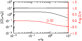
Asymptotecan draw secondary axes with the routinespicture secondaryX(picture primary=currentpicture, void f(picture)); picture secondaryY(picture primary=currentpicture, void f(picture));
In this example,
secondaryYis used to draw a secondary linear y axis against a primary logarithmic y axis:import graph; texpreamble("\def\Arg{\mathop {\rm Arg}\nolimits}"); size(10cm,5cm,IgnoreAspect); real ampl(real x) {return 2.5/sqrt(1+x^2);} real phas(real x) {return -atan(x)/pi;} scale(Log,Log); draw(graph(ampl,0.01,10)); ylimits(0.001,100); xaxis("$\omega\tau_0$",BottomTop,LeftTicks); yaxis("$|G(\omega\tau_0)|$",Left,RightTicks); picture q=secondaryY(new void(picture pic) { scale(pic,Log,Linear); draw(pic,graph(pic,phas,0.01,10),red); ylimits(pic,-1.0,1.5); yaxis(pic,"$\Arg G/\pi$",Right,red, LeftTicks("$% #.1f$", begin=false,end=false)); yequals(pic,1,Dotted); }); label(q,"(1,0)",Scale(q,(1,0)),red); add(q);
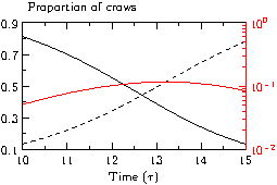
A secondary logarithmic y axis can be drawn like this:
import graph;

size(9cm,6cm,IgnoreAspect);
string data="secondaryaxis.csv";

file in=input(data).line().csv();

string[] titlelabel=in;
string[] columnlabel=in;

real[][] a=in;
a=transpose(a);
real[] t=a[0], susceptible=a[1], infectious=a[2], dead=a[3], larvae=a[4];
real[] susceptibleM=a[5], exposed=a[6], infectiousM=a[7];

scale(true);

draw(graph(t,susceptible,t >= 10 & t <= 15));
draw(graph(t,dead,t >= 10 & t <= 15),dashed);

xaxis("Time ($\tau$)",BottomTop,LeftTicks);
yaxis(Left,RightTicks);

picture secondary=secondaryY(new void(picture pic) {
    scale(pic,Linear(true),Log(true));
    draw(pic,graph(pic,t,infectious,t >= 10 & t <= 15),red);
    yaxis(pic,Right,red,LeftTicks(begin=false,end=false));
  });

add(secondary);
label(shift(5mm*N)*"Proportion of crows",point(NW),E);
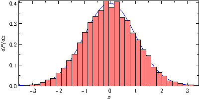
- Here is a histogram example, which uses the
statsmodule.import graph; import stats; size(400,200,IgnoreAspect); int n=10000; real[] a=new real[n]; for(int i=0; i < n; ++i) a[i]=Gaussrand(); draw(graph(Gaussian,min(a),max(a)),blue); // Optionally calculate "optimal" number of bins a la Shimazaki and Shinomoto. int N=bins(a); histogram(a,min(a),max(a),N,normalize=true,low=0,lightred,black,bars=true); xaxis("$x$",BottomTop,LeftTicks); yaxis("$dP/dx$",LeftRight,RightTicks(trailingzero));
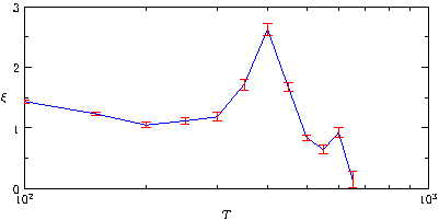
- Here is an example of reading column data in from a file and a
least-squares fit, using the
statsmodule.size(400,200,IgnoreAspect); import graph; import stats; file fin=input("leastsquares.dat").line(); real[][] a=fin; a=transpose(a); real[] t=a[0], rho=a[1]; // Read in parameters from the keyboard: //real first=getreal("first"); //real step=getreal("step"); //real last=getreal("last"); real first=100; real step=50; real last=700; // Remove negative or zero values of rho: t=rho > 0 ? t : null; rho=rho > 0 ? rho : null; scale(Log(true),Linear(true)); int n=step > 0 ? ceil((last-first)/step) : 0; real[] T,xi,dxi; for(int i=0; i <= n; ++i) { real first=first+i*step; real[] logrho=(t >= first & t <= last) ? log(rho) : null; real[] logt=(t >= first & t <= last) ? -log(t) : null; if(logt.length < 2) break; // Fit to the line logt=L.m*logrho+L.b: linefit L=leastsquares(logt,logrho); T.push(first); xi.push(L.m); dxi.push(L.dm); } draw(graph(T,xi),blue); errorbars(T,xi,dxi,red); crop(); ylimits(0); xaxis("$T$",BottomTop,LeftTicks); yaxis("$\xi$",LeftRight,RightTicks);
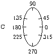
- Here is an example that illustrates the general
axisroutine.import graph; size(0,100); path g=ellipse((0,0),1,2); scale(true); axis(Label("C",align=10W),g,LeftTicks(endlabel=false,8,end=false), ticklocate(0,360,new real(real v) { path h=(0,0)--max(abs(max(g)),abs(min(g)))*dir(v); return intersect(g,h)[0];}));
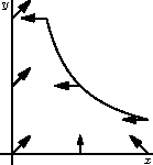
- To draw a vector field of
narrows evenly spaced along the arclength of a path, use the routinepicture vectorfield(path vector(real), path g, int n, bool truesize=false, pen p=currentpen, arrowbar arrow=Arrow);as illustrated in this simple example of a flow field:
import graph;
defaultpen(1.0);

size(0,150,IgnoreAspect);

real arrowsize=4mm;
real arrowlength=2arrowsize;

typedef path vector(real);

// Return a vector interpolated linearly between a and b.
vector vector(pair a, pair b) {
  return new path(real x) {
    return (0,0)--arrowlength*interp(a,b,x);
  };
}

real f(real x) {return 1/x;}

real epsilon=0.5;
path g=graph(f,epsilon,1/epsilon);

int n=3;
draw(g);
xaxis("$x$");
yaxis("$y$");

add(vectorfield(vector(W,W),g,n,true));
add(vectorfield(vector(NE,NW),(0,0)--(point(E).x,0),n,true));
add(vectorfield(vector(NE,NE),(0,0)--(0,point(N).y),n,true));
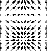
- To draw a vector field of
nx\timesnyarrows inbox(a,b), use the routinepicture vectorfield(path vector(pair), pair a, pair b, int nx=nmesh, int ny=nx, bool truesize=false, real maxlength=truesize ? 0 : maxlength(a,b,nx,ny), bool cond(pair z)=null, pen p=currentpen, arrowbar arrow=Arrow, margin margin=PenMargin)as illustrated in this example:
import graph;
size(100);

pair a=(0,0);
pair b=(2pi,2pi);

path vector(pair z) {return (sin(z.x),cos(z.y));}

add(vectorfield(vector,a,b));
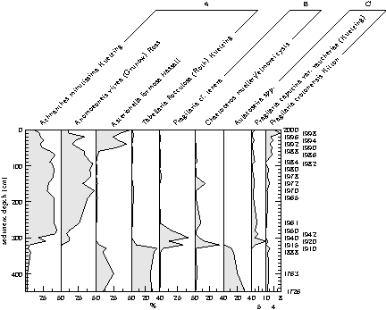
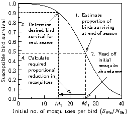
- The following scientific graphs, which illustrate many features of
Asymptote’s graphics routines, were generated from the examplesdiatom.asyandwestnile.asy, using the comma-separated data indiatom.csvandwestnile.csv.