---

3.5 Paths

This example draws a path that approximates a quarter circle, terminated with an arrowhead:

size(100,0);
draw((1,0){up}..{left}(0,1),Arrow);

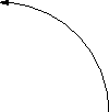
Here the directions up and left in braces specify the outgoing and incoming directions at the points (1,0) and (0,1), respectively.

In general, a path is specified as a list of points (or other paths) interconnected with --, which denotes a straight line segment, or .., which denotes a cubic spline (see Bezier curves). Specifying a final ..cycle creates a cyclic path that connects smoothly back to the initial node, as in this approximation (accurate to within 0.06%) of a unit circle:

path unitcircle=E..N..W..S..cycle;

An Asymptote path, being connected, is equivalent to a PostScript subpath. The ^^ binary operator, which requests that the pen be moved (without drawing or affecting endpoint curvatures) from the final point of the left-hand path to the initial point of the right-hand path, may be used to group several Asymptote paths into a path[] array (equivalent to a PostScript path):

size(0,100);
path unitcircle=E..N..W..S..cycle;
path g=scale(2)*unitcircle;
filldraw(unitcircle^^g,evenodd+yellow,black);

The PostScript even-odd fill rule here specifies that only the region bounded between the two unit circles is filled (see fillrule). In this example, the same effect can be achieved by using the default zero winding number fill rule, if one is careful to alternate the orientation of the paths:

filldraw(unitcircle^^reverse(g),yellow,black);

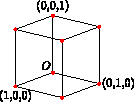
The ^^ operator is used by the box(triple, triple) function in the module three to construct the edges of a cube unitbox without retracing steps (see three):

import three;

currentprojection=orthographic(5,4,2,center=true);

size(5cm);
size3(3cm,5cm,8cm);

draw(unitbox);

dot(unitbox,red);

label("$O$",(0,0,0),NW);
label("(1,0,0)",(1,0,0),S);
label("(0,1,0)",(0,1,0),E);
label("(0,0,1)",(0,0,1),Z);

See section graph (or the online Asymptote gallery and external links posted at https://asymptote.sourceforge.io) for further examples, including two-dimensional and interactive three-dimensional scientific graphs. Additional examples have been posted by Philippe Ivaldi at https://web.archive.org/web/20201130113133/http://www.piprime.fr/asymptote.