---

8.29 three ¶

This module fully extends the notion of guides and paths in Asymptote to three dimensions. It introduces the new types guide3, path3, and surface. Guides in three dimensions are specified with the same syntax as in two dimensions except that triples (x,y,z) are used in place of pairs (x,y) for the nodes and direction specifiers. This generalization of John Hobby’s spline algorithm is shape-invariant under three-dimensional rotation, scaling, and shifting, and reduces in the planar case to the two-dimensional algorithm used in Asymptote, MetaPost, and MetaFont [see J. C. Bowman, Proceedings in Applied Mathematics and Mechanics, 7:1, 2010021-2010022 (2007)].

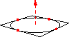
For example, a unit circle in the XY plane may be filled and drawn like this:

import three;

size(100);

path3 g=(1,0,0)..(0,1,0)..(-1,0,0)..(0,-1,0)..cycle;
draw(g);
draw(O--Z,red+dashed,Arrow3);
draw(((-1,-1,0)--(1,-1,0)--(1,1,0)--(-1,1,0)--cycle));
dot(g,red);

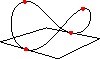
and then distorted into a saddle:

import three;

size(100,0);
path3 g=(1,0,0)..(0,1,1)..(-1,0,0)..(0,-1,1)..cycle;
draw(g);
draw(((-1,-1,0)--(1,-1,0)--(1,1,0)--(-1,1,0)--cycle));
dot(g,red);

Module three provides constructors for converting two-dimensional paths to three-dimensional ones, and vice-versa:

path3 path3(path p, triple plane(pair)=XYplane);
path path(path3 p, pair P(triple)=xypart);

A Bezier surface, the natural two-dimensional generalization of Bezier curves, is defined in three_surface.asy as a structure containing an array of Bezier patches. Surfaces may drawn with one of the routines

void draw(picture pic=currentpicture, surface s, int nu=1, int nv=1,
          material surfacepen=currentpen, pen meshpen=nullpen,
          light light=currentlight, light meshlight=nolight, string name="",
          render render=defaultrender);
void draw(picture pic=currentpicture, surface s, int nu=1, int nv=1,
          material[] surfacepen, pen meshpen,
          light light=currentlight, light meshlight=nolight, string name="",
          render render=defaultrender);
void draw(picture pic=currentpicture, surface s, int nu=1, int nv=1,
          material[] surfacepen, pen[] meshpen=nullpens,
          light light=currentlight, light meshlight=nolight, string name="",
          render render=defaultrender);

The parameters nu and nv specify the number of subdivisions for drawing optional mesh lines for each Bezier patch. The optional name parameter is used as a prefix for naming the surface patches in the PRC model tree. Here material is a structure defined in three_light.asy:

struct material {
  pen[] p; // diffusepen,emissivepen,specularpen
  real opacity;
  real shininess;
  real metallic;
  real fresnel0;
}

These material properties are used to implement physically based rendering (PBR) using light properties defined in plain_prethree.asy and three_light.asy:

struct light {
  real[][] diffuse;
  real[][] specular;
  pen background=nullpen; // Background color of the canvas.
  real specularfactor;
  triple[] position; // Only directional lights are currently implemented.
}

light Viewport=light(specularfactor=3,(0.25,-0.25,1));

light White=light(new pen[] {rgb(0.38,0.38,0.45),rgb(0.6,0.6,0.67),
                             rgb(0.5,0.5,0.57)},specularfactor=3,
  new triple[] {(-2,-1.5,-0.5),(2,1.1,-2.5),(-0.5,0,2)});

light Headlamp=light(gray(0.8),specular=gray(0.7),
                     specularfactor=3,dir(42,48));

currentlight=Headlamp;

light nolight;

The currentlight.background (or background member of the specified light) can be used to set the background color for 2D (or 3D) images. The default background is white for HTML images and transparent for all other formats. One can request a completely transparent background for 3D WebGL images with currentlight.background=black+opacity(0.0);

render

A function render() may be assigned to the optional render parameter allows one to pass specialized rendering options to the surface drawing routines, via arguments such as:

  bool tessellate;   // use tessellated mesh to store straight patches
  real margin;       // shrink amount for rendered OpenGL viewport, in bp.
  bool partnames;    // assign part name indices to compound objects
  bool defaultnames; // assign default names to unnamed objects
  interaction interaction; // billboard interaction mode

along with the rendering parameters for the legacy PRC format described in three.asy.

Asymptote also supports image-based lighting with the setting settings.ibl=true. This uses pre-rendered EXR images from the directory specified by -imageDir (which defaults to ibl) or, for WebGL rendering, the URL specified by -imageURL (which defaults to https://vectorgraphics.gitlab.io/asymptote/ibl). Additional rendered images can be generated on an NVIDIA GPU using the reflect program in the cudareflect subdirectory of the Asymptote source directory.

Sample Bezier surfaces are contained in the example files BezierSurface.asy, teapot.asy, teapotIBL.asy, and parametricsurface.asy.

The structure render contains specialized rendering options documented at the beginning of module three.

The examples elevation.asy and sphericalharmonic.asy illustrate how to draw a surface with patch-dependent colors. The examples vertexshading.asy and smoothelevation.asy illustrate vertex-dependent colors, which are supported by Asymptote’s native OpenGL/WebGL renderers and the two-dimensional vector output format (settings.render=0). Since the legacy PRC output format does not support vertex shading of Bezier surfaces, PRC patches are shaded with the mean of the four vertex colors.

A surface can be constructed from a cyclic path3 with the constructor

surface surface(path3 external, triple[] internal=new triple[],
                pen[] colors=new pen[], bool3 planar=default);

and then filled:

draw(surface(unitsquare3,new triple[] {X,Y,Z,O}),red);
draw(surface(O--X{Y}..Y{-X}--cycle,new triple[] {Z}),red);
draw(surface(path3(polygon(5))),red,nolight);
draw(surface(unitcircle3),red,nolight);
draw(surface(unitcircle3,new pen[] {red,green,blue,black}),nolight);

The first example draws a Bezier patch and the second example draws a Bezier triangle. The third and fourth examples are planar surfaces. The last example constructs a patch with vertex-specific colors. A three-dimensional planar surface in the plane plane can be constructed from a two-dimensional cyclic path g with the constructor

surface surface(path p, triple plane(pair)=XYplane);

and then filled:

draw(surface((0,0)--E+2N--2E--E+N..0.2E..cycle),red);

Planar Bezier surfaces patches are constructed using Orest Shardt’s bezulate routine, which decomposes (possibly nonsimply connected) regions bounded (according to the zerowinding fill rule) by simple cyclic paths (intersecting only at the endpoints) into subregions bounded by cyclic paths of length 4 or less.

A more efficient routine also exists for drawing tessellations composed of many 3D triangles, with specified vertices, and optional normals or vertex colors:

void draw(picture pic=currentpicture, triple[] v, int[][] vi,
          triple[] n={}, int[][] ni=vi, material m=currentpen, pen[] p={},
          int[][] pi=vi, light light=currentlight);

Here, the triple array v lists the (typically distinct) vertices, while the array vi contains integer arrays of length 3 containing the indices of the elements in v that form the vertices of each triangle. Similarly, the arguments n and ni contain optional normal data and p and pi contain optional pen vertex data. If more than one normal or pen is specified for a vertex, the last one is used. An example of this tessellation facility is given in triangles.asy.

Arbitrary thick three-dimensional curves and line caps (which the OpenGL standard does not require implementations to provide) are constructed with

tube tube(path3 p, real width, render render=defaultrender);

this returns a tube structure representing a tube of diameter width centered approximately on g. The tube structure consists of a surface s and the actual tube center, path3 center. Drawing thick lines as tubes can be slow to render, especially with the Adobe Reader renderer. The setting thick=false can be used to disable this feature and force all lines to be drawn with linewidth(0) (one pixel wide, regardless of the resolution). By default, mesh and contour lines in three-dimensions are always drawn thin, unless an explicit line width is given in the pen parameter or the setting thin is set to false. The pens thin() and thick() defined in plain_pens.asy can also be used to override these defaults for specific draw commands.

There are six choices for viewing 3D Asymptote output:

1. Use the native Asymptote adaptive OpenGL-based renderer (with the command-line option -V and the default settings outformat="" and render=-1). On UNIX systems with graphics support for multisampling, the sample width can be controlled with the setting multisample. The ratio of physical to logical screen pixels can be specified with the setting devicepixelratio. An initial screen position can be specified with the pair setting position, where negative values are interpreted as relative to the corresponding maximum screen dimension. The default settings

   import settings;
   leftbutton=new string[] {"rotate","zoom","shift","pan"};
   middlebutton=new string[] {""};
   rightbutton=new string[] {"zoom","rotateX","rotateY","rotateZ"};
   wheelup=new string[] {"zoomin"};
   wheeldown=new string[] {"zoomout"};
   

   bind the mouse buttons as follows:

   • Left: rotate
   • Shift Left: zoom
   • Ctrl Left: shift viewport
   • Alt Left: pan
   • Wheel Up: zoom in
   • Wheel Down: zoom out
   • Right: zoom
   • Shift Right: rotate about the X axis
   • Ctrl Right: rotate about the Y axis
   • Alt Right: rotate about the Z axis

   The keyboard bindings are:

   • h: home
   • f: toggle fitscreen
   • x: spin about the X axis
   • y: spin about the Y axis
   • z: spin about the Z axis
   • s: stop spinning
   • m: rendering mode (solid/patch/mesh)
   • e: export
   • c: show camera parameters
   • p: play animation
   • r: reverse animation
   • : step animation
   • +: expand
   • =: expand
   • >: expand
   • -: shrink
   • _: shrink
   • <: shrink
   • q: exit
   • Ctrl-q: exit
2. Generate WebGL interactive vector graphics output with the the command-line option and -f html (or the setting outformat="html"). The resulting 3D HTML file can then be viewed directly in any modern desktop or mobile browser, or even embedded within another web page:

   <iframe src="logo3.html" width="561" height="321" frameborder="0">
   </iframe>
   

   Normally, WebGL files generated by Asymptote are dynamically remeshed to fit the browser window dimensions. However, the setting absolute=true can be used to force the image to be rendered at its designed size (accounting for multiple device pixels per css pixel).

   For specialized applications, the setting keys=true can be used to generate an identifying key immediately before the WebGL code for each generated object. The default key, the "line:column" of the associated function call of the top-level source code, can be overwritten by adding KEY="x" as the first argument of the function call, where x represents user-supplied text.

   The interactive WebGL files produced by Asymptote use the default mouse and (many of the same) key bindings as the OpenGL renderer. Zooming via the mouse wheel of a WebGL image embedded within another page is disabled until the image is activated by a click or touch event and will remain enabled until the ESC key is pressed.

   By default, viewing the 3D HTML files generated by Asymptote requires network access to download the AsyGL rendering library, which is normally cached by the browser for future use. However, the setting offline=true can be used to embed this small (about 48kB) library within a stand-alone HTML file that can be viewed offline.

3. Render the scene to a specified rasterized format outformat at the resolution of n pixels per bp, as specified by the setting render=n. A negative value of n is interpreted as |2n| for EPS and PDF formats and |n| for other formats. The default value of render is -1. By default, the scene is internally rendered at twice the specified resolution; this can be disabled by setting antialias=1. High resolution rendering is done by tiling the image. If your graphics card allows it, the rendering can be made more efficient by increasing the maximum tile size maxtile to your screen dimensions (indicated by maxtile=(0,0). If your video card generates unwanted black stripes in the output, try setting the horizontal and vertical components of maxtiles to something less than your screen dimensions. The tile size is also limited by the setting maxviewport, which restricts the maximum width and height of the viewport. Some graphics drivers support batch mode (-noV) rendering in an iconified window; this can be enabled with the setting iconify=true.
4. Embed the 3D legacy PRC format in a PDF file and view the resulting PDF file with version 9.0 or later of Adobe Reader. This requires settings.outformat="pdf" and settings.prc=true, which can be specified by the command-line options -f pdf and -f prc, put in the Asymptote configuration file (see configuration file), or specified in the script before module three (or graph3) is imported. The media9 LaTeX package is also required (see embed). The example 100d.asy illustrates how one can generate a list of predefined views (see 100d.views). A stationary preview image with a resolution of n pixels per bp can be embedded with the setting render=n; this allows the file to be viewed with other PDF viewers. Alternatively, the file externalprc.tex illustrates how the resulting PRC and rendered image files can be extracted and processed in a separate LaTeX file. However, see LaTeX usage for an easier way to embed three-dimensional Asymptote pictures within LaTeX. For specialized applications where only the raw PRC file is required, specify settings.outformat="prc". The PRC specification is available from https://web.archive.org/web/20081204104459/http://livedocs.adobe.com/acrobat_sdk/9/Acrobat9_HTMLHelp/API_References/PRCReference/PRC_Format_Specification/
5. Output a V3D portable compressed vector graphics file using settings.outformat="v3d", which can be viewed with an external viewer or converted to an alternate 3D format using the Python pyv3d library. V3D content can be automatically embedded within a PDF file using the options settings.outformat="pdf" and settings.v3d=true. Alternatively, a V3D file file.v3d may be manually embedded within a PDF file using the media9 LaTeX package:

   \includemedia[noplaybutton,width=100pt,height=200pt]{}{file.v3d}%
   

   An online Javascript-based V3D-aware PDF viewer is available at https://github.com/vectorgraphics/pdfv3dReader.

   The V3D specification and the pyv3d library are available at https://github.com/vectorgraphics/v3d. A V3D file file.v3d may be imported and viewed by Asymptote either by specifying file.v3d on the command line

   asy -V file.v3d
   

   or using the v3d module and importv3d function in interactive mode (or within an Asymptote file):

   import v3d;
   importv3d("file.v3d");
   

6. Project the scene to a two-dimensional vector (EPS or PDF) format with render=0. Only limited support for hidden surface removal, lighting, and transparency is available with this approach (see PostScript3D).

Automatic picture sizing in three dimensions is accomplished with double deferred drawing. The maximal desired dimensions of the scene in each of the three dimensions can optionally be specified with the routine

void size3(picture pic=currentpicture, real x, real y=x, real z=y,
          bool keepAspect=pic.keepAspect);

A simplex linear programming problem is then solved to produce a 3D version of a frame (actually implemented as a 3D picture). The result is then fit with another application of deferred drawing to the viewport dimensions corresponding to the usual two-dimensional picture size parameters. The global pair viewportmargin may be used to add horizontal and vertical margins to the viewport dimensions. Alternatively, a minimum viewportsize may be specified. A 3D picture pic can be explicitly fit to a 3D frame by calling

frame pic.fit3(projection P=currentprojection);

and then added to picture dest about position with

void add(picture dest=currentpicture, frame src, triple position=(0,0,0));

For convenience, the three module defines O=(0,0,0), X=(1,0,0), Y=(0,1,0), and Z=(0,0,1), along with a unitcircle in the XY plane:

path3 unitcircle3=X..Y..-X..-Y..cycle;

A general (approximate) circle can be drawn perpendicular to the direction normal with the routine

path3 circle(triple c, real r, triple normal=Z);

A circular arc centered at c with radius r from c+r*dir(theta1,phi1) to c+r*dir(theta2,phi2), drawing counterclockwise relative to the normal vector cross(dir(theta1,phi1),dir(theta2,phi2)) if theta2 > theta1 or if theta2 == theta1 and phi2 >= phi1, can be constructed with

path3 arc(triple c, real r, real theta1, real phi1, real theta2, real phi2,
          triple normal=O);

The normal must be explicitly specified if c and the endpoints are colinear. If r < 0, the complementary arc of radius |r| is constructed. For convenience, an arc centered at c from triple v1 to v2 (assuming |v2-c|=|v1-c|) in the direction CCW (counter-clockwise) or CW (clockwise) may also be constructed with

path3 arc(triple c, triple v1, triple v2, triple normal=O,
          bool direction=CCW);

When high accuracy is needed, the routines Circle and Arc defined in graph3 may be used instead. See GaussianSurface for an example of a three-dimensional circular arc.

The representation O--O+u--O+u+v--O+v--cycle of the plane passing through point O with normal cross(u,v) is returned by

path3 plane(triple u, triple v, triple O=O);

A three-dimensional box with opposite vertices at triples v1 and v2 may be drawn with the function

path3[] box(triple v1, triple v2);

For example, a unit box is predefined as

path3[] unitbox=box(O,(1,1,1));

Asymptote also provides optimized definitions for the three-dimensional paths unitsquare3 and unitcircle3, along with the surfaces unitdisk, unitplane, unitcube, unitcylinder, unitcone, unitsolidcone, unitfrustum(real t1, real t2), unitsphere, and unithemisphere.

These projections to two dimensions are predefined:

oblique

oblique(real angle) ¶

The point (x,y,z) is projected to (x-0.5z,y-0.5z). If an optional real argument is given, the negative z axis is drawn at this angle in degrees. The projection obliqueZ is a synonym for oblique.

obliqueX

obliqueX(real angle) ¶

The point (x,y,z) is projected to (y-0.5x,z-0.5x). If an optional real argument is given, the negative x axis is drawn at this angle in degrees.

obliqueY

obliqueY(real angle) ¶

The point (x,y,z) is projected to (x+0.5y,z+0.5y). If an optional real argument is given, the positive y axis is drawn at this angle in degrees.

orthographic(triple camera, triple up=Z, triple target=O,
             real zoom=1, pair viewportshift=0, bool showtarget=true,
             bool center=true) ¶

This projects from three to two dimensions using the view as seen at a point infinitely far away in the direction unit(camera), orienting the camera so that, if possible, the vector up points upwards. Parallel lines are projected to parallel lines. The bounding volume is expanded to include target if showtarget=true. If center=true, the target will be adjusted to the center of the bounding volume.

orthographic(real x, real y, real z, triple up=Z, triple target=O,
             real zoom=1, pair viewportshift=0, bool showtarget=true,
             bool center=true)

This is equivalent to

orthographic((x,y,z),up,target,zoom,viewportshift,showtarget,center)

The routine

triple camera(real alpha, real beta);

can be used to compute the camera position with the x axis below the horizontal at angle alpha, the y axis below the horizontal at angle beta, and the z axis up.

perspective(triple camera, triple up=Z, triple target=O,
            real zoom=1, real angle=0, pair viewportshift=0,
            bool showtarget=true, bool autoadjust=true,
            bool center=autoadjust) ¶

This projects from three to two dimensions, taking account of perspective, as seen from the location camera looking at target, orienting the camera so that, if possible, the vector up points upwards. If autoadjust=true, the camera will automatically be adjusted to lie outside the bounding volume for all possible interactive rotations about target. If center=true, the target will be adjusted to the center of the bounding volume.

perspective(real x, real y, real z, triple up=Z, triple target=O,
            real zoom=1, real angle=0, pair viewportshift=0,
            bool showtarget=true, bool autoadjust=true,
            bool center=autoadjust)

This is equivalent to

perspective((x,y,z),up,target,zoom,angle,viewportshift,showtarget,
            autoadjust,center)

The default projection, currentprojection, is initially set to perspective(5,4,2).

We also define standard orthographic views used in technical drawing:

projection LeftView=orthographic(-X,showtarget=true);
projection RightView=orthographic(X,showtarget=true);
projection FrontView=orthographic(-Y,showtarget=true);
projection BackView=orthographic(Y,showtarget=true);
projection BottomView=orthographic(-Z,showtarget=true);
projection TopView=orthographic(Z,showtarget=true);

The function

void addViews(picture dest=currentpicture, picture src,
              projection[][] views=SixViewsUS,
              bool group=true, filltype filltype=NoFill);

adds to picture dest an array of views of picture src using the layout projection[][] views. The default layout SixViewsUS aligns the projection FrontView below TopView and above BottomView, to the right of LeftView and left of RightView and BackView. The predefined layouts are:

projection[][] ThreeViewsUS={{TopView},
                             {FrontView,RightView}};

projection[][] SixViewsUS={{null,TopView},
                           {LeftView,FrontView,RightView,BackView},
                           {null,BottomView}};

projection[][] ThreeViewsFR={{RightView,FrontView},
                             {null,TopView}};

projection[][] SixViewsFR={{null,BottomView},
                           {RightView,FrontView,LeftView,BackView},
                           {null,TopView}};

projection[][] ThreeViews={{FrontView,TopView,RightView}};

projection[][] SixViews={{FrontView,TopView,RightView},
                         {BackView,BottomView,LeftView}};

A triple or path3 can be projected to a pair or path, with project(triple, projection P=currentprojection) or project(path3, projection P=currentprojection).

It is occasionally useful to be able to invert a projection, sending a pair z onto the plane perpendicular to normal and passing through point:

triple invert(pair z, triple normal, triple point,
              projection P=currentprojection);

A pair z on the projection plane can be inverted to a triple with the routine

triple invert(pair z, projection P=currentprojection);

A pair direction dir on the projection plane can be inverted to a triple direction relative to a point v with the routine

triple invert(pair dir, triple v, projection P=currentprojection).

Three-dimensional objects may be transformed with one of the following built-in transform3 types (the identity transformation is identity4):

shift(triple v) ¶

translates by the triple v;

xscale3(real x) ¶

scales by x in the x direction;

yscale3(real y) ¶

scales by y in the y direction;

zscale3(real z) ¶

scales by z in the z direction;

scale3(real s) ¶

scales by s in the x, y, and z directions;

scale(real x, real y, real z) ¶

scales by x in the x direction, by y in the y direction, and by z in the z direction;

rotate(real angle, triple v)

rotates by angle in degrees about the axis O--v;

rotate(real angle, triple u, triple v)

rotates by angle in degrees about the axis u--v;

reflect(triple u, triple v, triple w)

reflects about the plane through u, v, and w.

When not multiplied on the left by a transform3, three-dimensional TeX Labels are drawn as Bezier surfaces directly on the projection plane:

void label(picture pic=currentpicture, Label L, triple position,
           align align=NoAlign, pen p=currentpen,
           light light=nolight, string name="",
           render render=defaultrender, interaction interaction=
           settings.autobillboard ? Billboard : Embedded)

The optional name parameter is used as a prefix for naming the label patches in the PRC model tree. The default interaction is Billboard, which means that labels are rotated interactively so that they always face the camera. The interaction Embedded means that the label interacts as a normal 3D surface, as illustrated in the example billboard.asy. Alternatively, a label can be transformed from the XY plane by an explicit transform3 or mapped to a specified two-dimensional plane with the predefined transform3 types XY, YZ, ZX, YX, ZY, ZX. There are also modified versions of these transforms that take an optional argument projection P=currentprojection that rotate and/or flip the label so that it is more readable from the initial viewpoint.

A transform3 that projects in the direction dir onto the plane with normal n through point O is returned by

transform3 planeproject(triple n, triple O=O, triple dir=n);

One can use

triple normal(path3 p);

to find the unit normal vector to a planar three-dimensional path p. As illustrated in the example planeproject.asy, a transform3 that projects in the direction dir onto the plane defined by a planar path p is returned by

transform3 planeproject(path3 p, triple dir=normal(p));

The functions

surface extrude(path p, triple axis=Z);
surface extrude(Label L, triple axis=Z);

return the surface obtained by extruding path p or Label L along axis.

Three-dimensional versions of the path functions length, size, point, dir, accel, radius, precontrol, postcontrol, arclength, arctime, reverse, subpath, intersect, intersections, intersectionpoint, intersectionpoints, min, max, cyclic, and straight are also defined.

The routine

real[] intersect(path3 p, surface s, real fuzz=-1);

returns a real array of length 3 containing the intersection times, if any, of a path p with a surface s. The routine

real[][] intersections(path3 p, surface s, real fuzz=-1);

returns all (unless there are infinitely many) intersection times of a path p with a surface s as a sorted array of real arrays of length 3, and

triple[] intersectionpoints(path3 p, surface s, real fuzz=-1);

returns the corresponding intersection points. Here, the computations are performed to the absolute error specified by fuzz, or if fuzz < 0, to machine precision. The routine

real orient(triple a, triple b, triple c, triple d);

is a numerically robust computation of dot(cross(a-d,b-d),c-d), which is the determinant

|a.x a.y a.z 1|
|b.x b.y b.z 1|
|c.x c.y c.z 1|
|d.x d.y d.z 1|

The result is negative (positive) if a, b, c appear in counterclockwise (clockwise) order when viewed from d or zero if all four points are coplanar.

The routine

real insphere(triple a, triple b, triple c, triple d, triple e);

returns a positive (negative) value if e lies inside (outside) the sphere passing through points a,b,c,d oriented so that dot(cross(a-d,b-d),c-d) is positive, or zero if all five points are cospherical. The value returned is the determinant

|a.x a.y a.z a.x^2+a.y^2+a.z^2 1|
|b.x b.y b.z b.x^2+b.y^2+b.z^2 1|
|c.x c.y c.z c.x^2+c.y^2+c.z^2 1|
|d.x d.y d.z d.x^2+d.y^2+d.z^2 1|
|e.x e.y e.z e.x^2+e.y^2+e.z^2 1|

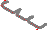
Here is an example showing all five guide3 connectors:

import graph3;

size(200);

currentprojection=orthographic(500,-500,500);

triple[] z=new triple[10];

z[0]=(0,100,0); z[1]=(50,0,0); z[2]=(180,0,0);

for(int n=3; n <= 9; ++n)
  z[n]=z[n-3]+(200,0,0);

path3 p=z[0]..z[1]---z[2]::{Y}z[3]
&z[3]..z[4]--z[5]::{Y}z[6]
&z[6]::z[7]---z[8]..{Y}z[9];

draw(p,grey+linewidth(4mm),currentlight);

xaxis3(Label(XY()*"$x$",align=-3Y),red,above=true);
yaxis3(Label(XY()*"$y$",align=-3X),red,above=true);

Three-dimensional versions of bars or arrows can be drawn with one of the specifiers None, Blank, BeginBar3, EndBar3 (or equivalently Bar3), Bars3, BeginArrow3, MidArrow3, EndArrow3 (or equivalently Arrow3), Arrows3, BeginArcArrow3, EndArcArrow3 (or equivalently ArcArrow3), MidArcArrow3, and ArcArrows3. Three-dimensional bars accept the optional arguments (real size=0, triple dir=O). If size=O, the default bar length is used; if dir=O, the bar is drawn perpendicular to the path and the initial viewing direction. The predefined three-dimensional arrowhead styles are DefaultHead3, HookHead3, TeXHead3. Versions of the two-dimensional arrowheads lifted to three-dimensional space and aligned according to the initial viewpoint (or an optionally specified normal vector) are also defined: DefaultHead2(triple normal=O), HookHead2(triple normal=O), TeXHead2(triple normal=O). These are illustrated in the example arrows3.asy.

Module three also defines the three-dimensional margins NoMargin3, BeginMargin3, EndMargin3, Margin3, Margins3, BeginPenMargin2, EndPenMargin2, PenMargin2, PenMargins2, BeginPenMargin3, EndPenMargin3, PenMargin3, PenMargins3, BeginDotMargin3, EndDotMargin3, DotMargin3, DotMargins3, Margin3, and TrueMargin3.

The routine

void pixel(picture pic=currentpicture, triple v, pen p=currentpen,
           real width=1);

can be used to draw on picture pic a pixel of width width at position v using pen p.

Further three-dimensional examples are provided in the files near_earth.asy, conicurv.asy, and (in the animations subdirectory) cube.asy.

Limited support for projected vector graphics (effectively three-dimensional nonrendered PostScript) is available with the setting render=0. This currently only works for piecewise planar surfaces, such as those produced by the parametric surface routines in the graph3 module. Surfaces produced by the solids module will also be properly rendered if the parameter nslices is sufficiently large.

In the module bsp, hidden surface removal of planar pictures is implemented using a binary space partition and picture clipping. A planar path is first converted to a structure face derived from picture. A face may be given to a two-dimensional drawing routine in place of any picture argument. An array of such faces may then be drawn, removing hidden surfaces:

void add(picture pic=currentpicture, face[] faces,
         projection P=currentprojection);

Labels may be projected to two dimensions, using projection P, onto the plane passing through point O with normal cross(u,v) by multiplying it on the left by the transform

transform transform(triple u, triple v, triple O=O,
                    projection P=currentprojection);

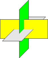
Here is an example that shows how a binary space partition may be used to draw a two-dimensional vector graphics projection of three orthogonal intersecting planes:

size(6cm,0);
import bsp;

real u=2.5;
real v=1;

currentprojection=oblique;

path3 y=plane((2u,0,0),(0,2v,0),(-u,-v,0));
path3 l=rotate(90,Z)*rotate(90,Y)*y;
path3 g=rotate(90,X)*rotate(90,Y)*y;

face[] faces;
filldraw(faces.push(y),project(y),yellow);
filldraw(faces.push(l),project(l),lightgrey);
filldraw(faces.push(g),project(g),green);

add(faces);